Ficheiro:Conjugate gradient illustration.svg

Dimensões desta antevisão em PNG do ficheiro SVG: 398 × 600 píxeis Outras resoluções: 159 × 240 píxeis | 318 × 480 píxeis | 509 × 768 píxeis | 679 × 1 024 píxeis | 1 358 × 2 048 píxeis | 804 × 1 212 píxeis.
Ficheiro original (ficheiro SVG, de 804 × 1 212 píxeis, tamanho: 2 kB)
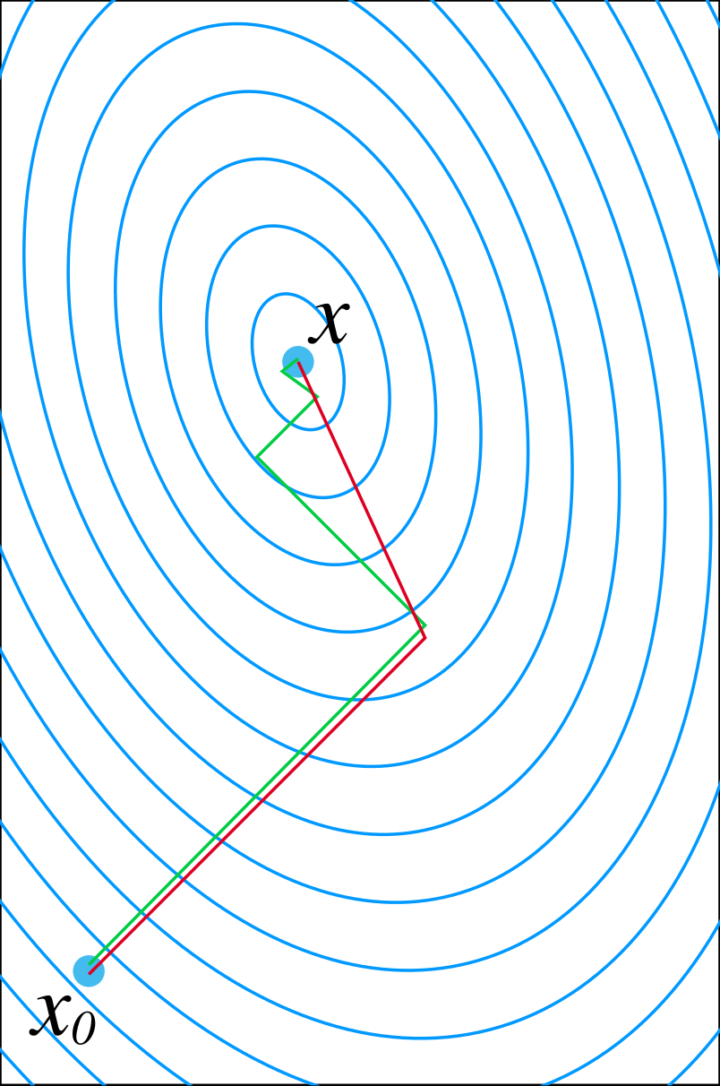
| Descrição | Illustration of en:Conjugate gradient method |
| Data | (UTC) |
| Origem | self-made, with en:Matlab, and then tweaked in en:Inkscape |
| Autor | Oleg Alexandrov |
| Eu, titular dos direitos de autor desta obra, dedico-a ao domínio público, com aplicação em todo o mundo. Nalguns países isto pode não ser legalmente possível; se assim for: Concedo a todos o direito de usar esta obra para qualquer fim, sem quaisquer condições, a menos que tais condições sejam impostas por lei. |
Source code (MATLAB)
% A comparision of gradient descent and conjugate gradient (guess who wins)

function main()

   % data
   A=[17, 2; 2, 7];  % the matrix
   b=[2, 2]';        % right-hand side
   x0=[0, 0]';       % the initial guess

   % linewidth and font size
   lw= 2;
   fs = 25;

% colors
   red=[0.867 0.06 0.14];
   blue = [0, 129, 205]/256;
   green = [0, 200,  70]/256;
   black = [0, 0, 0];
   white = 0.99*[1, 1, 1];

   % Set up the plotting window
   figure(1); clf; set(gca, 'fontsize', fs); hold on; axis equal; axis off;
   s = 0.16; x = A\b;
   Ax = x(1)-s; Bx = x(1)+s; Ay = x(2)-2.0*s; By =  x(2)+s;
   plot([Ax Bx Bx Ax Ax], [Ay Ay By By Ay], 'color', blue, 'linewidth', lw/2); % plot a blue box
   s=0.005; plot(Ax-s, Ay-s, '*', 'color', white); plot(Bx+0.5*s, By+0.5*s, '*', 'color', white); %markers
   Box = [Ax Bx Ay By];
   axis (Box);

   % plot the contours of the quadratic form associated with A and b
   plot_contours(A, b, Box, lw, blue);

% Do conjugate gradient and gradient descent.
% For the first one, start a bit shifted so that the two graphs don't overlap.
   shift = 0.0015*[1, -1];
   small_rad=0.002;
   tol = eps;
   x = conj_gradient(A, b, x0, tol, lw, red,   small_rad,  shift);
   x = grad_descent (A, b, x0, tol, lw, green, small_rad);

% text
   small = 0.015;
   text(x0(1)-2*small, x0(2)-1.6*small, 'x', 'fontsize', fs);
   text(x0(1)-0.5*small, x0(2)-3*small, '0', 'fontsize', floor(0.7*fs));
   text(x(1)+small, x(2)+small, 'x', 'fontsize', fs);

% some balls for beauty
   small_rad = 0.003;
   ball(x0(1)+shift(1)/2, x0(2)+shift(2)/2, small_rad, blue)
   ball(x(1), x(2), small_rad, blue)

% save to disk as eps and svg
   saveas(gcf, 'Conjugate_gradient_illustration.eps', 'psc2');
   plot2svg('Conjugate_gradient_illustration.svg');


function x = conj_gradient(A, b, x, tol, lw, color, small_rad, shift)

   r=A*x - b;
   d=-r;

   while norm(r) > tol

      % a pretty ball for beauty, to cover imperfections when two segments are joined
      ball(x(1)+shift(1), x(2)+shift(2), small_rad, color);

      alpha = -dot(r, d)/dot(A*d, d);
      x0 = x;
      x = x + alpha*d;

      r=A*x - b;
      beta = dot(A*r, d)/dot(A*d, d);
      d0 = d;
      d = -r + beta*d;

      plot([x0(1), x(1)]+shift(1), [x0(2), x(2)]+shift(2), 'color', color, 'linewidth', lw)

   end

function x = grad_descent(A, b, x, tol, lw, color, small_rad)

   r=A*x - b;
   d=-r;

   while norm(r) > tol

      % a pretty ball for beauty, to cover imperfections when two segments are joined
      ball(x(1), x(2), small_rad, color);

      alpha = -dot(r, d)/dot(A*d, d);
      x0 = x;
      x = x + alpha*d;

      r=A*x - b;
      beta = 0; %beta = dot(A*r, d)/dot(A*d, d);
      d0 = d;
      d = -r + beta*d;

      plot([x0(1), x(1)], [x0(2), x(2)], 'color', color, 'linewidth', lw)

   end


function plot_contours (A, b, Box, lw, color);

   N=200;  % number of points (don't make it big, code will be slow)

   E = A\b; % the exact solution, around which we will draw the contours
   B = 0.12;
   [X, Y]=meshgrid(linspace(Box(1)-B, Box(2)+B, N), linspace(Box(3)-B, Box(4)+B, N));     % X and Y coordinates

% the quadratic form f= (1/2)*x'*A*X-b'*x;
   f = inline('0.5*A(1, 1)*X.*X + A(1, 2)*X.*Y+0.5*A(2, 2)*Y.*Y-b(1)*X-b(2)*Y', 'X', 'Y', 'A', 'b');
   Z = 0.5*A(1, 1)*X.*X + A(1, 2)*X.*Y+0.5*A(2, 2)*Y.*Y-b(1)*X-b(2)*Y;


   % prepare to draw the contours
   x0 = A\b; f0 = f(x0(1), x0(2), A, b);
   No = 25; % number of contours
   Levels = (linspace(f0, 1, No)-f0).^2+f0;

% Plot the contours with 'contour' in figure(2), and then with 'plot' in figure(1).
% This is to avoid a bug in plot2svg, it can't save output of 'contour'.
   figure(2); clf; hold on;
   for i=1:length(Levels)

      figure(2);
      [c, stuff] = contour(X, Y, Z, [Levels(i), Levels(i)]);

      [m, n]=size(c);
      if m > 1 & n > 0

	 % extract the contour from the contour matrix and plot in figure(1)
	 l=c(2, 1);
	 x=c(1,2:(l+1));  y=c(2,2:(l+1));
	 figure(1); plot(x, y, 'color', color, 'linewidth', lw/2);

      end
   end
   figure(1);

function ball(x, y, r, color)
   Theta=0:0.1:2*pi;
   X=r*cos(Theta)+x;
   Y=r*sin(Theta)+y;
   H=fill(X, Y, color);
   set(H, 'EdgeColor', 'none');
Histórico do ficheiro
Clique uma data e hora para ver o ficheiro tal como ele se encontrava nessa altura.
| Data e hora | Miniatura | Dimensões | Utilizador | Comentário | |
|---|---|---|---|---|---|
| atual | 22h49min de 23 de março de 2024 | | 804 × 1 212 (2 kB) | Д.Ильин | Optimization |
| 01h49min de 20 de junho de 2007 |  | 606 × 900 (179 kB) | Oleg Alexandrov | {{Information |Description=Illustration of en:Conjugate gradient method |Source=self-made, with en:Matlab, and then tweaked in en:Inkscape |Date= ~~~~~ |Author= Oleg Alexandrov }} {{PD-self}} [[Category:Numerical a |
Utilização local do ficheiro
As seguintes 4 páginas usam este ficheiro:
Utilização global do ficheiro
As seguintes wikis usam este ficheiro:
- Uso no domínio de.wikipedia.org
- Uso no domínio en.wikipedia.org
- Uso no domínio fr.wikipedia.org
- Uso no domínio hu.wikipedia.org
- Uso no domínio ja.wikipedia.org
- Uso no domínio ko.wikipedia.org
- Uso no domínio pl.wikipedia.org
- Uso no domínio pt.wikipedia.org
- Uso no domínio ru.wikipedia.org
- Uso no domínio uk.wikipedia.org